1  Introduction

$$ \newcommand{\LetThereBe}[2]{\newcommand{#1}{#2}} \newcommand{\letThereBe}[3]{\newcommand{#1}[#2]{#3}} \newcommand{\ForceToBe}[2]{\renewcommand{#1}{#2}} \newcommand{\forceToBe}[3]{\renewcommand{#1}[#2]{#3}} \newcommand{\MayThereBe}[2]{\newcommand{#1}{#2}} \newcommand{\mayThereBe}[3]{\newcommand{#1}[#2]{#3}} % Declare mathematics (so they can be overwritten for PDF) \newcommand{\declareMathematics}[2]{\DeclareMathOperator{#1}{#2}} \newcommand{\declareMathematicsStar}[2]{\DeclareMathOperator*{#1}{#2}} % striked integral \newcommand{\avint}{\mathop{\mathchoice{\,\rlap{-}\!\!\int} {\rlap{\raise.15em{\scriptstyle -}}\kern-.2em\int} {\rlap{\raise.09em{\scriptscriptstyle -}}\!\int} {\rlap{-}\!\int}}\nolimits} % \d does not work well for PDFs \LetThereBe{\d}{\differential} \LetThereBe{\Im}{\IM} \LetThereBe{\Re}{\RE} \LetThereBe{\Cpls}{\mathrm{C{\scriptsize PL}}} \LetThereBe{\OptCpls}{\mathrm{O{\scriptsize pt}}} \letThereBe{\linefrac}{2}{#1/#2} \LetThereBe{\ExtProd}{\mathsf{\Lambda}} \letThereBe{\unicodeInt}{1}{\mathop{\vcenter{\mathchoice{\huge\unicode{#1}}{\unicode{#1}}{\unicode{#1}}{\unicode{#1}}}}\nolimits} \letThereBe{\Oiint}{1}{\underset{ #1 \;}{ {\rlap{\mspace{1mu} \boldsymbol{\bigcirc}}{\rlap{\int}{\;\int}}} }} \letThereBe{\sOiint}{1}{\unicodeInt{x222F}_{#1}} $$ $$ % Simply for testing \LetThereBe{\foo}{\textrm{FIXME: this is a test!}} % Font styles \letThereBe{\mcal}{1}{\mathcal{#1}} \letThereBe{\chem}{1}{\mathrm{#1}} % Sets \LetThereBe{\C}{\mathbb{C}} \LetThereBe{\R}{\mathbb{R}} \LetThereBe{\Z}{\mathbb{Z}} \LetThereBe{\N}{\mathbb{N}} \LetThereBe{\Q}{\mathbb{Q}} \LetThereBe{\K}{\mathbb{K}} \LetThereBe{\im}{\mathrm{i}} % Sets from PDEs \LetThereBe{\boundaryOf}{\partial} \letThereBe{\closureOf}{1}{\overline{#1}} \letThereBe{\Contf}{1}{\mcal C^{#1}} \letThereBe{\contf}{2}{\Contf{#2}(#1)} \letThereBe{\compactContf}{2}{\mcal C_c^{#2}(#1)} \letThereBe{\ball}{2}{B\brackets{#1, #2}} \letThereBe{\closedBall}{2}{B\parentheses{#1, #2}} \LetThereBe{\compactEmbed}{\subset\subset} \letThereBe{\inside}{1}{#1^o} \LetThereBe{\neighborhood}{\mcal O} \letThereBe{\neigh}{1}{\neighborhood \brackets{#1}} % Basic notation - vectors and random variables \letThereBe{\vi}{1}{\boldsymbol{#1}} %vector or matrix \letThereBe{\dvi}{1}{\vi{\dot{#1}}} %differentiated vector or matrix \letThereBe{\vii}{1}{\mathbf{#1}} %if \vi doesn't work \letThereBe{\dvii}{1}{\vii{\dot{#1}}} %if \dvi doesn't work \letThereBe{\rnd}{1}{\mathup{#1}} %random variable \letThereBe{\vr}{1}{\mathbf{#1}} %random vector or matrix \letThereBe{\vrr}{1}{\boldsymbol{#1}} %random vector if \vr doesn't work \letThereBe{\dvr}{1}{\vr{\dot{#1}}} %differentiated vector or matrix \letThereBe{\vb}{1}{\pmb{#1}} %#TODO \letThereBe{\dvb}{1}{\vb{\dot{#1}}} %#TODO \letThereBe{\oper}{1}{\mathsf{#1}} \letThereBe{\quotient}{2}{{^{\displaystyle #1}}/{_{\displaystyle #2}}} % Basic notation - general \letThereBe{\set}{1}{\left\{#1\right\}} \letThereBe{\seqnc}{4}{\set{#1_{#2}}_{#2 = #3}^{#4}} \letThereBe{\Seqnc}{3}{\set{#1}_{#2}^{#3}} \letThereBe{\brackets}{1}{\left( #1 \right)} \letThereBe{\parentheses}{1}{\left[ #1 \right]} \letThereBe{\dom}{1}{\mcal{D}\, \brackets{#1}} \letThereBe{\complexConj}{1}{\overline{#1}} \LetThereBe{\divider}{\; \vert \;} \LetThereBe{\gets}{\leftarrow} \letThereBe{\rcases}{1}{\left.\begin{aligned}#1\end{aligned}\right\}} \letThereBe{\rcasesAt}{2}{\left.\begin{alignedat}{#1}#2\end{alignedat}\right\}} \letThereBe{\lcases}{1}{\begin{cases}#1\end{cases}} \letThereBe{\lcasesAt}{2}{\left\{\begin{alignedat}{#1}#2\end{alignedat}\right.} \letThereBe{\evaluateAt}{2}{\left.#1\right|_{#2}} \LetThereBe{\Mod}{\;\mathrm{mod}\;} \LetThereBe{\bigO}{O} \letThereBe{\BigO}{1}{\bigO\brackets{#1}} % Special symbols \LetThereBe{\const}{\mathrm{const}} \LetThereBe{\konst}{\mathrm{konst.}} \LetThereBe{\vf}{\varphi} \LetThereBe{\ve}{\varepsilon} \LetThereBe{\tht}{\theta} \LetThereBe{\Tht}{\Theta} \LetThereBe{\after}{\circ} \LetThereBe{\lmbd}{\lambda} \LetThereBe{\Lmbd}{\Lambda} % Shorthands \LetThereBe{\xx}{\vi x} \LetThereBe{\yy}{\vi y} \LetThereBe{\AA}{\vi A} \LetThereBe{\bb}{\vi b} \LetThereBe{\vvf}{\vi \vf} \LetThereBe{\ff}{\vi f} \LetThereBe{\gg}{\vi g} % Basic functions \letThereBe{\absval}{1}{\left| #1 \right|} \LetThereBe{\id}{\mathrm{id}} \letThereBe{\floor}{1}{\left\lfloor #1 \right\rfloor} \letThereBe{\ceil}{1}{\left\lceil #1 \right\rceil} \declareMathematics{\image}{im} %image \declareMathematics{\domain}{dom} %image \declareMathematics{\tg}{tg} \declareMathematics{\sign}{sign} \declareMathematics{\card}{card} %cardinality \letThereBe{\setSize}{1}{\left| #1 \right|} \LetThereBe{\countElements}{\#} \declareMathematics{\exp}{exp} \letThereBe{\Exp}{1}{\exp\brackets{#1}} \LetThereBe{\ee}{\mathrm{e}} \letThereBe{\indicator}{1}{\mathbb{I}_{#1}} \declareMathematics{\arccot}{arccot} \declareMathematics{\gcd}{gcd} % Greatest Common Divisor \declareMathematics{\lcm}{lcm} % Least Common Multiple \declareMathematics{\epi}{epi} %epigraph of a function \letThereBe{\limInfty}{1}{\lim_{#1 \to \infty}} \letThereBe{\limInftyM}{1}{\lim_{#1 \to -\infty}} % Useful commands \letThereBe{\onTop}{2}{\mathrel{\overset{#2}{#1}}} \letThereBe{\onBottom}{2}{\mathrel{\underset{#2}{#1}}} \letThereBe{\tOnTop}{2}{\mathrel{\overset{\text{#2}}{#1}}} \letThereBe{\tOnBottom}{2}{\mathrel{\underset{\text{#2}}{#1}}} \LetThereBe{\EQ}{\onTop{=}{!}} \LetThereBe{\letDef}{:=} %#TODO: change the symbol \LetThereBe{\isPDef}{\onTop{\succ}{?}} \LetThereBe{\inductionStep}{\tOnTop{=}{induct. step}} \LetThereBe{\fromDef}{\triangleq} % Optimization \declareMathematicsStar{\argmin}{argmin} \declareMathematicsStar{\argmax}{argmax} \letThereBe{\maxOf}{1}{\max\set{#1}} \letThereBe{\minOf}{1}{\min\set{#1}} \declareMathematics{\prox}{prox} \declareMathematics{\loss}{loss} \declareMathematics{\supp}{supp} \letThereBe{\Supp}{1}{\supp\brackets{#1}} \LetThereBe{\constraint}{\text{s.t.}\;} $$ $$ % Operators - Analysis \LetThereBe{\hess}{\nabla^2} \LetThereBe{\lagr}{\mcal L} \LetThereBe{\lapl}{\Delta} \declareMathematics{\grad}{grad} \declareMathematics{\divergence}{div} \declareMathematics{\Dgrad}{D} \LetThereBe{\gradient}{\nabla} \LetThereBe{\jacobi}{\nabla} \LetThereBe{\Jacobi}{\vi{\mathrm J}} \letThereBe{\jacobian}{2}{\Dgrad_{#1}\brackets{#2}} \LetThereBe{\d}{\mathrm{d}} \LetThereBe{\dd}{\,\mathrm{d}} \letThereBe{\partialDeriv}{2}{\frac {\partial #1} {\partial #2}} \letThereBe{\npartialDeriv}{3}{\partialDeriv{^{#1} #2} {#3^{#1}}} \letThereBe{\partialOp}{1}{\frac {\partial} {\partial #1}} \letThereBe{\npartialOp}{2}{\frac {\partial^{#1}} {\partial #2^{#1}}} \letThereBe{\pDeriv}{2}{\partialDeriv{#1}{#2}} \letThereBe{\npDeriv}{3}{\npartialDeriv{#1}{#2}{#3}} \letThereBe{\deriv}{2}{\frac {\d #1} {\d #2}} \letThereBe{\nderiv}{3}{\frac {\d^{#1} #2} {\d #3^{#1}}} \letThereBe{\derivOp}{1}{\frac {\d} {\d #1}\,} \letThereBe{\nderivOp}{2}{\frac {\d^{#1}} {\d #2^{#1}}\,} % Convergence \LetThereBe{\pointwiseTo}{\to} \LetThereBe{\uniformlyTo}{\rightrightarrows} \LetThereBe{\normallyTo}{\tOnTop{\longrightarrow}{norm}} \LetThereBe{\compactlyTo}{\tOnTop{\longrightarrow}{comp.}} \LetThereBe{\locallyUnifTo}{\tOnTop{\longrightarrow}{l.u.}} % Curves \letThereBe{\graphOf}{1}{\parentheses{#1}} \declareMathematics{\interior}{Int} % complex \LetThereBe{\Cinfty}{\tilde{\C}} \declareMathematics{\residual}{res} \letThereBe{\resAt}{1}{\residual_{#1}} \declareMathematics{\complexarg}{arg} \declareMathematics{\complexArg}{Arg} \LetThereBe{\carg}{\complexarg} \LetThereBe{\cArg}{\complexArg} \LetThereBe{\IM}{\mathfrak{Im}} \LetThereBe{\RE}{\mathfrak{Re}} \letThereBe{\imOf}{1}{\IM\,#1} \letThereBe{\reOf}{1}{\RE\,#1} \letThereBe{\ImOf}{1}{\IM \brackets{#1}} \letThereBe{\ReOf}{1}{\RE \brackets{#1}} % Convex \letThereBe{\cconj}{1}{#1^*} $$ $$ % Linear algebra \letThereBe{\norm}{1}{\left\lVert #1 \right\rVert} \letThereBe{\seminorm}{1}{{\left\vert\kern-0.25ex\left\vert\kern-0.25ex\left\vert #1 \right\vert\kern-0.25ex\right\vert\kern-0.25ex\right\vert}} \letThereBe{\scal}{2}{\left\langle #1, #2 \right\rangle} \letThereBe{\avg}{1}{\overline{#1}} \letThereBe{\Avg}{1}{\bar{#1}} \letThereBe{\linspace}{1}{\mathrm{lin}\set{#1}} \letThereBe{\algMult}{1}{\mu_{\mathrm A} \brackets{#1}} \letThereBe{\geomMult}{1}{\mu_{\mathrm G} \brackets{#1}} \LetThereBe{\Nullity}{\mathrm{nullity}} \letThereBe{\nullity}{1}{\Nullity \brackets{#1}} \LetThereBe{\nulty}{\nu} \declareMathematics{\SpanOf}{span} \letThereBe{\Span}{1}{\SpanOf\set{#1}} \LetThereBe{\projection}{\Pi} % Linear algebra - Matrices \LetThereBe{\tr}{\top} \LetThereBe{\Tr}{^\tr} \LetThereBe{\pinv}{\dagger} \LetThereBe{\Pinv}{^\dagger} \LetThereBe{\Inv}{^{-1}} \LetThereBe{\ident}{\vi{I}} \letThereBe{\mtr}{1}{\begin{pmatrix}#1\end{pmatrix}} \letThereBe{\bmtr}{1}{\begin{bmatrix}#1\end{bmatrix}} \declareMathematics{\trace}{tr} \declareMathematics{\diagonal}{diag} \declareMathematics{\rank}{rank} % Multilinear algebra \LetThereBe{\tensorProd}{\otimes} \LetThereBe{\tprod}{\tensorProd} \LetThereBe{\extProd}{\wedge} \LetThereBe{\wdg}{\extProd} \LetThereBe{\wedges}{\wedge \dots \wedge} \declareMathematics{\altMap}{Alt} $$ $$ % Statistics \LetThereBe{\iid}{\overset{\text{i.i.d.}}{\sim}} \LetThereBe{\ind}{\overset{\text{ind}}{\sim}} \LetThereBe{\condp}{\,\vert\,} \letThereBe{\complementOf}{1}{{#1^{\mathrm{c}}}} \LetThereBe{\acov}{\gamma} \LetThereBe{\acf}{\rho} \LetThereBe{\stdev}{\sigma} \LetThereBe{\procMean}{\mu} \LetThereBe{\procVar}{\stdev^2} \declareMathematics{\variance}{var} \letThereBe{\Variance}{1}{\variance \brackets{#1}} \declareMathematics{\cov}{cov} \declareMathematics{\corr}{cor} \letThereBe{\sampleVar}{1}{\rnd S^2_{#1}} \letThereBe{\populationVar}{1}{V_{#1}} \declareMathematics{\expectedValue}{\mathbb{E}} \declareMathematics{\rndMode}{Mode} \letThereBe{\RndMode}{1}{\rndMode\brackets{#1}} \letThereBe{\expect}{1}{\expectedValue #1} \letThereBe{\Expect}{1}{\expectedValue \brackets{#1}} \letThereBe{\expectIn}{2}{\expectedValue_{#1} #2} \letThereBe{\ExpectIn}{2}{\expectedValue_{#1} \brackets{#2}} \LetThereBe{\betaF}{\mathrm B} \LetThereBe{\fisherMat}{J} \LetThereBe{\mutInfo}{I} \LetThereBe{\expectedGain}{I_e} \letThereBe{\KLDiv}{2}{D\brackets{#1 \parallel #2}} \LetThereBe{\entropy}{H} \LetThereBe{\diffEntropy}{h} \LetThereBe{\probF}{\pi} \LetThereBe{\densF}{\vf} \LetThereBe{\att}{_t} %at time \letThereBe{\estim}{1}{\hat{#1}} \letThereBe{\estimML}{1}{\hat{#1}_{\mathrm{ML}}} \letThereBe{\estimOLS}{1}{\hat{#1}_{\mathrm{OLS}}} \letThereBe{\estimMAP}{1}{\hat{#1}_{\mathrm{MAP}}} \letThereBe{\predict}{3}{\estim {\rnd #1}_{#2 | #3}} \letThereBe{\periodPart}{3}{#1+#2-\ceil{#2/#3}#3} \letThereBe{\infEstim}{1}{\tilde{#1}} \letThereBe{\predictDist}{1}{{#1}^*} \LetThereBe{\backs}{\oper B} \LetThereBe{\diff}{\oper \Delta} \LetThereBe{\BLP}{\oper P} \LetThereBe{\arPoly}{\Phi} \letThereBe{\ArPoly}{1}{\arPoly\brackets{#1}} \LetThereBe{\maPoly}{\Theta} \letThereBe{\MaPoly}{1}{\maPoly\brackets{#1}} \letThereBe{\ARmod}{1}{\mathrm{AR}\brackets{#1}} \letThereBe{\MAmod}{1}{\mathrm{MA}\brackets{#1}} \letThereBe{\ARMA}{2}{\mathrm{ARMA}\brackets{#1, #2}} \letThereBe{\sARMA}{3}{\mathrm{ARMA}\brackets{#1}\brackets{#2}_{#3}} \letThereBe{\SARIMA}{3}{\mathrm{ARIMA}\brackets{#1}\brackets{#2}_{#3}} \letThereBe{\ARIMA}{3}{\mathrm{ARIMA}\brackets{#1, #2, #3}} \LetThereBe{\pacf}{\alpha} \letThereBe{\parcorr}{3}{\rho_{#1 #2 | #3}} \LetThereBe{\noise}{\mathscr{N}} \LetThereBe{\jeffreys}{\mathcal J} \LetThereBe{\likely}{\mcal L} \letThereBe{\Likely}{1}{\likely\brackets{#1}} \LetThereBe{\loglikely}{\mcal l} \letThereBe{\Loglikely}{1}{\loglikely \brackets{#1}} \LetThereBe{\CovMat}{\Gamma} \LetThereBe{\covMat}{\vi \CovMat} \LetThereBe{\rcovMat}{\vrr \CovMat} \LetThereBe{\AIC}{\mathrm{AIC}} \LetThereBe{\BIC}{\mathrm{BIC}} \LetThereBe{\AICc}{\mathrm{AIC}_c} \LetThereBe{\nullHypo}{H_0} \LetThereBe{\altHypo}{H_1} \LetThereBe{\rve}{\rnd \ve} \LetThereBe{\rtht}{\rnd \theta} \LetThereBe{\rX}{\rnd X} \LetThereBe{\rY}{\rnd Y} \LetThereBe{\rZ}{\rnd Z} \LetThereBe{\rA}{\rnd A} \LetThereBe{\rB}{\rnd B} \LetThereBe{\rU}{\rnd U} \LetThereBe{\vrZ}{\vr Z} \LetThereBe{\vrY}{\vr Y} \LetThereBe{\vrX}{\vr X} \LetThereBe{\vrU}{\vr U} \LetThereBe{\rW}{\rnd W} \LetThereBe{\rS}{\rnd S} \LetThereBe{\rM}{\rnd M} \LetThereBe{\rtau}{\rnd \tau} % Bayesian inference \LetThereBe{\paramSet}{\mcal T} \LetThereBe{\sampleSet}{\mcal Y} \LetThereBe{\bayesSigmaAlg}{\mcal B} % Different types of convergence \LetThereBe{\inDist}{\onTop{\to}{d}} \letThereBe{\inDistWhen}{1}{\onBottom{\onTop{\longrightarrow}{d}}{#1}} \LetThereBe{\inProb}{\onTop{\to}{P}} \letThereBe{\inProbWhen}{1}{\onBottom{\onTop{\longrightarrow}{P}}{#1}} \LetThereBe{\inMeanSq}{\onTop{\to}{\ltwo}} \LetThereBe{\inltwo}{\onTop{\to}{\ltwo}} \letThereBe{\inMeanSqWhen}{1}{\onBottom{\onTop{\longrightarrow}{\ltwo}}{#1}} \LetThereBe{\convergeAS}{\tOnTop{\to}{a.s.}} \letThereBe{\convergeASWhen}{1}{\onBottom{\tOnTop{\longrightarrow}{a.s.}}{#1}} % Asymptotic qualities \LetThereBe{\simAsymp}{\tOnTop{\sim}{as.}} % Stochastic analysis \letThereBe{\diffOn}{2}{\diff #1_{[#2]}} % \LetThereBe{\timeSet}{\Theta} \LetThereBe{\eventSet}{\Omega} \LetThereBe{\filtration}{\mcal F} % TODO: Rename allFiltrations and the like \letThereBe{\allFiltrations}{1}{\set{\filtration_t}_{#1}} \letThereBe{\natFilter}{1}{\filtration_t^{#1}} \letThereBe{\NatFilter}{2}{\filtration_{#2}^{#1}} \letThereBe{\filterAll}{1}{\set{#1}_{t \geq 0}} \letThereBe{\FilterAll}{2}{\set{#1}_{#2}} \LetThereBe{\borelAlgebra}{\mcal B} \LetThereBe{\sAlgebra}{\mcal A} \LetThereBe{\quadVar}{Q} \LetThereBe{\totalVar}{V} \LetThereBe{\adaptIntProcs}{\mcal M} \letThereBe{\reflectProc}{2}{#1^{#2}} $$ $$ % Distributions \letThereBe{\WN}{2}{\mathrm{WN}\brackets{#1,#2}} \declareMathematics{\uniform}{Unif} \declareMathematics{\binomDist}{Bi} \declareMathematics{\negbinomDist}{NBi} \declareMathematics{\betaDist}{Beta} \declareMathematics{\betabinomDist}{BetaBin} \declareMathematics{\gammaDist}{Gamma} \declareMathematics{\igammaDist}{IGamma} \declareMathematics{\invgammaDist}{IGamma} \declareMathematics{\expDist}{Ex} \declareMathematics{\poisDist}{Po} \declareMathematics{\erlangDist}{Er} \declareMathematics{\altDist}{A} \declareMathematics{\geomDist}{Ge} \LetThereBe{\normalDist}{\mathcal N} %\declareMathematics{\normalDist}{N} \letThereBe{\normalD}{1}{\normalDist \brackets{#1}} \letThereBe{\mvnormalD}{2}{\normalDist_{#1} \brackets{#2}} \letThereBe{\NormalD}{2}{\normalDist \brackets{#1, #2}} \LetThereBe{\lognormalDist}{\log\normalDist} $$ $$ % Game Theory \LetThereBe{\doms}{\succ} \LetThereBe{\isdom}{\prec} \letThereBe{\OfOthers}{1}{_{-#1}} \LetThereBe{\ofOthers}{\OfOthers{i}} \LetThereBe{\pdist}{\sigma} \letThereBe{\domGame}{1}{G_{DS}^{#1}} \letThereBe{\ratGame}{1}{G_{Rat}^{#1}} \letThereBe{\bestRep}{2}{\mathrm{BR}_{#1}\brackets{#2}} \letThereBe{\perf}{1}{{#1}_{\mathrm{perf}}} \LetThereBe{\perfG}{\perf{G}} \letThereBe{\imperf}{1}{{#1}_{\mathrm{imp}}} \LetThereBe{\imperfG}{\imperf{G}} \letThereBe{\proper}{1}{{#1}_{\mathrm{proper}}} \letThereBe{\finrep}{2}{{#2}_{#1{\text -}\mathrm{rep}}} %T-stage game \letThereBe{\infrep}{1}{#1_{\mathrm{irep}}} \LetThereBe{\repstr}{\tau} %strategy in a repeated game \LetThereBe{\emptyhist}{\epsilon} \letThereBe{\extrep}{1}{{#1^{\mathrm{rep}}}} \letThereBe{\avgpay}{1}{#1^{\mathrm{avg}}} \LetThereBe{\succf}{\pi} %successor function \LetThereBe{\playf}{\rho} %player function \LetThereBe{\actf}{\chi} %action function $$ $$ \LetThereBe{\fourierOp}{\mcal{F}} \letThereBe{\fourier}{1}{\widehat{#1}} \letThereBe{\ifourier}{1}{\check{#1}} % Shortcuts \letThereBe{\FT}{1}{\fourier{#1}} \letThereBe{\iFT}{1}{\ifourier{#1}} \LetThereBe{\FTOp}{\fourierOp} \LetThereBe{\XX}{\mcal X} \LetThereBe{\YY}{\mcal Y} \LetThereBe{\cc}{\mathsf{c}} \LetThereBe{\lspace}{\mcal L} \LetThereBe{\lone}{\lspace^{1}} \letThereBe{\Lone}{1}{\lone\brackets{#1}} \LetThereBe{\ltwo}{\lspace^2} \letThereBe{\Ltwo}{1}{\ltwo\brackets{#1}} \letThereBe{\lp}{1}{\lspace^{#1}} \letThereBe{\Lp}{2}{\lp{#1}\brackets{#2}} \LetThereBe{\linfty}{\lspace^{\infty}} \letThereBe{\Linfty}{1}{\linfty\brackets{#1}} \LetThereBe{\ltwoEq}{\onTop{=}{\ltwo}} \letThereBe{\decayContf}{1}{\mcal C_0\brackets{#1}} \letThereBe{\cinftyContf}{1}{\mcal C^{\infty}_c\brackets{#1}} \LetThereBe{\bddMeasFs}{\mcal M_{\mathrm{b}}} \LetThereBe{\contBddFs}{\mcal C_{\mathrm{b}}} \LetThereBe{\contFs}{\mcal C} \LetThereBe{\Borel}{\mathscr{B}} \LetThereBe{\FinSignMeas}{\mathscr{M}} \LetThereBe{\Probs}{\mathscr{P}} \letThereBe{\probs}{1}{\Probs\brackets{#1}} \LetThereBe{\SCMProbs}{\Probs_2} \letThereBe{\scmProbs}{1}{\SCMProbs\brackets{#1}} \LetThereBe{\ACProbs}{\SCMProbs^{\mathrm{ac}}} \letThereBe{\acProbs}{1}{\ACProbs\brackets{#1}} \letThereBe{\pushforward}{2}{#1_{\sharp}#2} \letThereBe{\pf}{2}{\pushforward{#1}{#2}} \declareMathematics{\Law}{Law} \declareMathematics{\Project}{pr} \letThereBe{\project}{1}{\Project^{#1}} \letThereBe{\pr}{1}{\project{#1}} \declareMathematics{\TV}{TV} \letThereBe{\cpls}{1}{\Cpls\brackets{#1}} \letThereBe{\optCpls}{1}{\OptCpls\brackets{#1}} \LetThereBe{\OT}{\mathrm{OT}} \LetThereBe{\wasserstein}{\mcal W_2} \LetThereBe{\wsGrad}{\gradient_{\mcal W}} \LetThereBe{\csubseteq}{\onTop{\subseteq}{\mathrm{c}}} \LetThereBe{\bddsubseteq}{\onTop{\subseteq}{\mathrm{bdd}}} \letThereBe{\cTr}{1}{#1^{\cc}} \letThereBe{\cbTr}{1}{#1^{\overline{\cc}}} $$ $$ % ODEs \LetThereBe{\timeInt}{\mcal I} \LetThereBe{\stimeInt}{\mcal J} \LetThereBe{\Wronsk}{\mcal W} \letThereBe{\wronsk}{1}{\Wronsk \parentheses{#1}} \LetThereBe{\prufRadius}{\rho} \LetThereBe{\prufAngle}{\vf} \LetThereBe{\weyr}{\sigma} \LetThereBe{\linDifOp}{\mathsf{L}} \LetThereBe{\Hurwitz}{\vi H} \letThereBe{\hurwitz}{1}{\Hurwitz \brackets{#1}} % Cont. Models \LetThereBe{\dirac}{\delta} \LetThereBe{\torus}{\mathbb{T}} % PDEs % \avint -- defined in format-respective tex files \LetThereBe{\fundamental}{\Phi} \LetThereBe{\fund}{\fundamental} \letThereBe{\normaDeriv}{1}{\partialDeriv{#1}{\vec{n}}} \letThereBe{\volAvg}{2}{\avint_{\ball{#1}{#2}}} \LetThereBe{\VolAvg}{\volAvg{x}{\ve}} \letThereBe{\surfAvg}{2}{\avint_{\boundaryOf \ball{#1}{#2}}} \LetThereBe{\SurfAvg}{\surfAvg{x}{\ve}} \LetThereBe{\corrF}{\varphi^{\times}} \LetThereBe{\greenF}{G} \letThereBe{\reflect}{1}{\tilde{#1}} \LetThereBe{\conv}{*} \letThereBe{\dotP}{2}{#1 \cdot #2} \letThereBe{\translation}{1}{\tau_{#1}} \declareMathematics{\dist}{dist} \letThereBe{\regularizef}{1}{\eta_{#1}} \letThereBe{\fourier}{1}{\widehat{#1}} \letThereBe{\ifourier}{1}{\check{#1}} \LetThereBe{\fourierOp}{\mcal F} \LetThereBe{\ifourierOp}{\mcal F^{-1}} \letThereBe{\FourierOp}{1}{\fourierOp\set{#1}} \letThereBe{\iFourierOp}{1}{\ifourierOp\set{#1}} \LetThereBe{\laplaceOp}{\mcal L} \letThereBe{\LaplaceOp}{1}{\laplaceOp\set{#1}} \letThereBe{\Norm}{1}{\absval{#1}} % SINDy \LetThereBe{\Koop}{\mcal K} \letThereBe{\oneToN}{1}{\left[#1\right]} \LetThereBe{\meas}{\mathrm{m}} \LetThereBe{\stateLoss}{\mcal J} \LetThereBe{\lagrm}{p} % Stochastic analysis \LetThereBe{\RiemannInt}{(\mcal R)} \LetThereBe{\RiemannStieltjesInt}{(\mcal {R_S})} \LetThereBe{\LebesgueInt}{(\mcal L)} \LetThereBe{\ItoInt}{(\mcal I)} \LetThereBe{\Stratonovich}{\circ} \LetThereBe{\infMean}{\alpha} \LetThereBe{\infVar}{\beta} % Dynamical systems \LetThereBe{\nUnit}{\mathrm N} \LetThereBe{\timeUnit}{\mathrm T} % Masters thesis \LetThereBe{\evolOp}{\oper{\vf}} \letThereBe{\obj}{1}{\mathbb{#1}} \LetThereBe{\timeSet}{\obj T} \LetThereBe{\stateSpace}{\obj X} \LetThereBe{\contStateSpace}{\stateSpace_{C}} \LetThereBe{\orbit}{Or} \letThereBe{\Orbit}{1}{\orbit\brackets{#1}} \LetThereBe{\limitSet}{\obj \Lambda} \LetThereBe{\crossSection}{\obj \Sigma} \declareMathematics{\codim}{codim} % Left and right closed-or-open intervals \LetThereBe{\lco}{\langle} \LetThereBe{\rco}{\rangle} \letThereBe{\testInt}{1}{\mathrm{Int}_{#1}} \letThereBe{\evalOp}{1}{\oper{\eta}_{#1}} \LetThereBe{\nonzeroEl}{\bullet} \LetThereBe{\zeroEl}{\circ} \LetThereBe{\solOp}{\oper{S}} \LetThereBe{\infGen}{\oper{A}} \LetThereBe{\indexSet}{\mcal I} \letThereBe{\indicesOf}{1}{\indexSet\parentheses{#1}} \letThereBe{\IndicesOf}{2}{\indexSet_{#2}\parentheses{#1}} \LetThereBe{\meshGrid}{\obj M} \declareMathematics{\starter}{starter} \declareMathematics{\indexer}{indx} \declareMathematics{\enumerator}{enum} \LetThereBe{\inSS}{_{\infty}} \LetThereBe{\manifold}{\mcal M} \LetThereBe{\curve}{\mcal C} % Numerical methods \declareMathematics{\globErr}{err} \declareMathematics{\locErr}{le} \declareMathematics{\locTrErr}{lte} \declareMathematics{\estimErr}{est} \declareMathematics{\incrementFunc}{Inc} \letThereBe{\incrementF}{1}{\incrementFunc \brackets{#1}} \LetThereBe{\discreteNodes}{\mcal T} \LetThereBe{\stableFunc}{R} \letThereBe{\stableF}{1}{\stableFunc\brackets{#1}} \LetThereBe{\stableRegion}{\Omega} %Stochastic analysis \LetThereBe{\RiemannInt}{(\mcal R)} \LetThereBe{\RiemannStieltjesInt}{(\mcal {R_S})} \LetThereBe{\LebesgueInt}{(\mcal L)} \LetThereBe{\ItoInt}{(\mcal I)} \LetThereBe{\Stratonovich}{\circ} \LetThereBe{\infMean}{\alpha} \LetThereBe{\infVar}{\beta} %Optimization \LetThereBe{\goldRatio}{\tau} %Interpolation \LetThereBe{\lagrPoly}{l} $$

1.1 Motivation

Let us, for the moment, picture the Euclidean space \((\R^n, \absval{\cdot})\). Crucially, it is a complete separable metric space, i.e., a Polish space (see Definition 3.1), and it has a (simple) metric geometry together (geodesics and averages) with differential calculus. Can we do the same on probability measures?

Let \(\mu, \nu \in \probs{\R^d}\) be from the space of Borel probability measures on \(\R^d\).

Figure 1.1: Sketch of optimal transport for discrete measures

For single-point Dirac measure (both the source and target one), one can transport it by the geodesic in \(\R^d\). Alternatively, we could consider a linear average, see Figure 1.2.
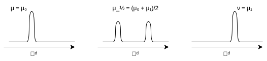
Figure 1.2: Linear average of Dirac measures

It turns out this is the geodesic with respect to the so-called total variation distance, see [1]. However, such transport does not take into account the geometry of the underlying base space!

Question 1.1: Distance of Probabilities

What is a natural distance on \(\probs{\R^d}\)?

Question 1.2: Geometry & Calculus of Probabilities

What is an appropriate metric geometry and differential calculus on \(\probs{\R^d}\)?

Let us start by considering the space of Dirac measures, i.e., \(\mu = \dirac_{\vi x}\), \(\nu = \dirac_{\vi y}\). The main idea will be to lift the geometry of \(\R^d\) to the space of probability measures \(d(\dirac_{\vi x}, \dirac_{\vi y}) := \absval{\vi x - \vi y}\). Similarly, we can define the average of \(\dirac_{\vi x}\) and \(\dirac_{\vi y}\) as \(\dirac_{\frac{\vi x + \vi y} 2}\). Can this be generalized?

1.1.1 Empirical Measures

Let us consider \(\mu, \nu\) to be convex combinations of Dirac measures, i.e., \[ \mu = \sum_{i = 1}^n \mu_i \dirac_{\vi x_i}, \quad \& \quad \nu = \sum_{j = 1}^m \nu_j \dirac_{\vi y_j}, \] and denote \(\mcal X := \set{\vi x_1, \dots, \vi x_n}\), \(\mcal Y := \set{\vi y_1, \dots, \vi y_m}\). The first (naive) idea is to transport “mass at \(\vi x_i\) to mass at \(\vi y_j\)”, i.e., define a transport map \(\vi T \colon \mcal X \to \mcal Y\) s.t. \[ \pf{\vi T}{\mu} = \sum_{i = 1}^n \mu_i \dirac_{\vi T(\vi x_i)} = \nu, \] where \(\pf{\vi T}{\mu}\) is the pushforward of \(\mu\) with respect to \(\vi T\). Surely, there are often many different transport maps (among which we must choose) and there exist various visualizations, see Figure 1.3.

(a) Transport map \(\vi T\) as pairings
(b) Graph of \(\vi T\)
Figure 1.3: Visualizations of a transport map \(\vi T\)

We follow up by another idea of selecting the “optimal” map by the “least action principle”. That is, we take a cost function \(\cc \colon \mcal X \times \mcal Y \to \R\). Given a transport map, it induces the corresponding transport cost \(\sum_{i = 1}^n \mu_i \cc(\vi x_i, \vi T(\vi x_i))\). This leads to the Monge formulation, \[ \inf_{\pf{\vi T}{\mu} = \nu} \sum_{i = 1}^n \mu_i \cc(\vi x_i, \vi T(\vi x_i)). \tag{1.1}\]

Caution

The Monge formulation is often ill-posed!

A way to relax from the Monge formulation (and avoid the ill-posedness) is to allow for mass-splitting, which leads to the Kantorovich (standard) formulation, see Figure 1.4.

(a) Non-Monge map \(\vi T\) as pairings
(b) Graph of \(\vi T\)
Figure 1.4: Visualizations of a non-Monge transport map \(\vi T\)

Indeed, consider the following Kantorovich optimal transport problem, \[ \begin{gathered} \inf_{\pi} \sum_{i,j = 1}^{n,m} \pi_{i,j} \cc(\vi x_i, \vi y_j), \; \text{ s.t. } \; \lcases{ \pi_{i,j} \geq 0, \\ \sum_{j = 1}^m \pi_{i,j} = \mu_i, \\ \sum_{i = 1}^n \pi_{i,j} = \nu_j. } \end{gathered} \tag{1.2}\] Note that the set of constraints is convex, compact and non-empty (e.g., \(\pi_{i,j} = \mu_i \cdot \nu_j\) satisfy the constraints). Thus, we have a standard linear programming problem! Moreover, one can make the following observations:

  1. The cost is linear in \(\pi\), hence there exists an optimizer1;
  2. Strong duality: (1.2) = (1.3), where \[ \sup_{(f_i)_i, (g_j)_j} \sum_{i = 1}^n \mu_i f_i + \sum_{j = 1}^m \nu_j g_j \; \text{ s.t. } \; f_i + g_j \leq \cc_{ij} = \cc(\vi x_i, \vi y_j) \tag{1.3}\] and \(f_i, g_j\) are Lagrange multipliers of the marginal constraints. Assume \((f,g)\) and \(\pi\) are admissible, then also weak-duality holds \[ \sum_{i = 1}^n f_i \mu_i + \sum_{j = 1}^m g_j \nu_j = \sum_{i,j = 1}^{n,m} \pi_{i,j} \underbrace{(f_i + g_j)}_{\leq \cc_{ij}} \leq \sum_{i,j = 1}^{n,m} \pi_{i,j} \cc_{i,j}; \]
  3. Complementary slackness: \((f,g)\) and \(\pi\) are optimal if and only if \(\pi_{i,j} > 0 \implies f_i + g_j = \cc_{ij}\);
  4. \(c\)-cyclical monotonicity: Let \(\pi\) be optimal, \(\Gamma = \supp \pi := \set{(\vi x_i, \vi y_j) \in \mcal X \times \mcal Y \mid \pi_{i,j} > 0}\). Then taking \((\hat{\vi x}_1, \hat{\vi y}_1), \dots, (\hat{\vi x}_k, \hat{\vi y}_k) \in \Gamma\) also gives \[ \sum_{i = 1}^k \cc(\hat{\vi x}_i, \hat{\vi y}_i) \leq \sum_{i = 1}^k \cc(\hat{\vi x}_i, \hat{\vi y}_{i+1}) \tag{1.4}\] with \(\hat{\vi y}_{k+1} = \hat{\vi y}_1\). In fact, \(\pi\) is optimal if and only if it is \(\cc\)-cyclically monotone, i.e., (1.4) holds. Let us show “\(\implies\)”. Indeed, for \(\pi\) optimal we also have \(f,g\) optimal for (1.3) and (3.) yields equality \(f(\hat{\vi x}_i) + g(\hat{\vi y}_i) = \cc(\hat{\vi x}_i, \hat{\vi y}_i)\) on the support. Thus summing over \(i\) gives us \[\begin{align*} \sum_{i = 1}^k \cc(\hat{\vi x}_i, \hat{\vi y}_i) &= \sum_{i = 1}^k f(\hat{\vi x}_i) + g(\hat{\vi y}_i) \\ &= \sum_{i = 1}^k f(\hat{\vi x}_i) + g(\hat{\vi y}_{i+1}) \\ &\leq \sum_{i = 1}^k \cc(\hat{\vi x}_i, \hat{\vi y}_{i+1}). \end{align*}\]

  1. Hence the cost is also continuous over a compact convex feasible set, thus we have existence.↩︎